I’ve long wanted to inject more live into my web presence and this blog in particular. It’s work in progress – one of my main sites is currently not even live! Wherever we may end up though, informal writing about science and the changing northern environment is something I want to do more of. So I’ve made two changes to give this site more oomph:
I’ve added a custom domain, borealperspectives.org, to this (currently) WordPress-hosted site. All URLs will work fine, whether you access them via borealperspetives.wordpress.com and the new borealperspectives.org. This is, unless and until I may decide in the future to move the site off WordPress.com, but that’s not in the stars right now.
I’ve moved to the smallest paid account to remove ads from the site. Only when I happened to access it from a browser that was not logged into WordPress.com did I see how intrusive the ads would be. It’s not much money, and I hope will make for more comfortable reading.
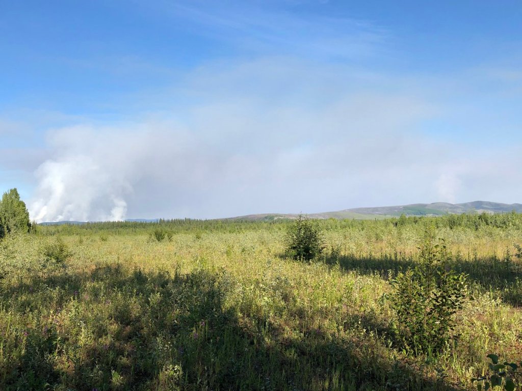
The numerous wildfires currently active in interior Alaska have made it a pretty miserable last day of the holiday weekend (Independence Day was Thursday in the US). The Fairbanks area is blanketed in smoke so badly that there’s a dense smoke advisory in effect and the local hospital has set up a smoke respite room for people with respiratory issues.
Most eyes are on the Shovel Creek fire NW of Fairbanks, which is burning very close to residential neighborhoods in mature black spruce forest, which naturally burns every ~100 years or so (plus/minus a large interval). It is managed by a Type 1 team – these are nationally managed in the US, and have the largest amount of experience and resources. There have been regular public information meetings, and the fire even has its own YouTube channel.
I live about 30 miles east of town, and over here, even though smoke these days comes from any of multiple fires in the wider area, the one we’re most concerned with is the Nugget Creek fire. It’s roughly the same order of magnitude as the Shovel Creek fire (a little smaller – 7000 acres / 2800 ha as of today, and growing – but unlike its companion, has not received any suppression activity at all, even though it’s only about 10 miles (16 km) from a residential area.
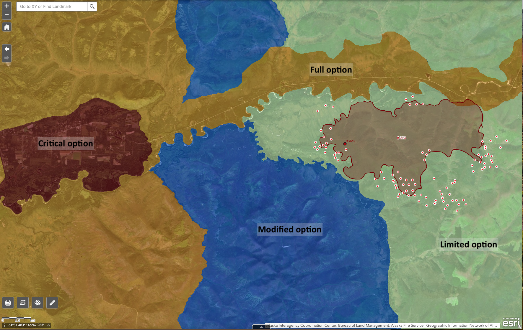
Why? This has to do with how decisions about fire management are made in Alaska. All of Alaska is divided into one of four fire management options. If you follow the link you’ll see that most of the remote areas are in the “limited” option. Here, fire is by default allowed to fulfill its natural ecological function, though known cabins and infrastructure is being protected by firefighters on the ground and from planes. Also, reconnaissance flights are being carried out, and fires are monitored. On the other extreme is the “critical” management option, where all fires are immediately suppressed. Towns and villages are covered by these. In-between, there are two intermediate options, “full” (covering the major road corridors, mining areas etc.) and “modified”. (These options are used for prioritization – there is no mechanical
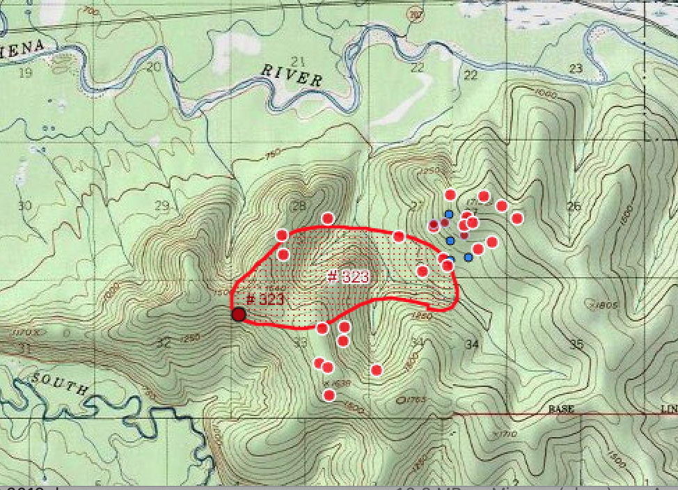
The Nugget Creek fire started in the Chena River State Recreation Area, in a location that is in the “limited management option. Here’s a map of the fire and how it is just nestled into the green, “limited” area. The fire is in red on the right, with the spots indicating where active fire was detected by satellite imagery. The fire has been pretty active on nearly its entire perimeter.
But it is still nearly entirely in the area that belongs to the limited management option. To the north, the full option starts at the Chena River and/or Chena Hot Springs Road, approximately. To the west, the modified option starts at the south fork of the Chena River (the confluence is where green, brown and blue areas meet). There are some fire service staff assigned to the fire, who have been continuously monitoring where the fire is relative to river/road in the north, and also have set up sprinklers to protect a public use cabin on the south fork of the Chena River (Nugget Creek cabin).
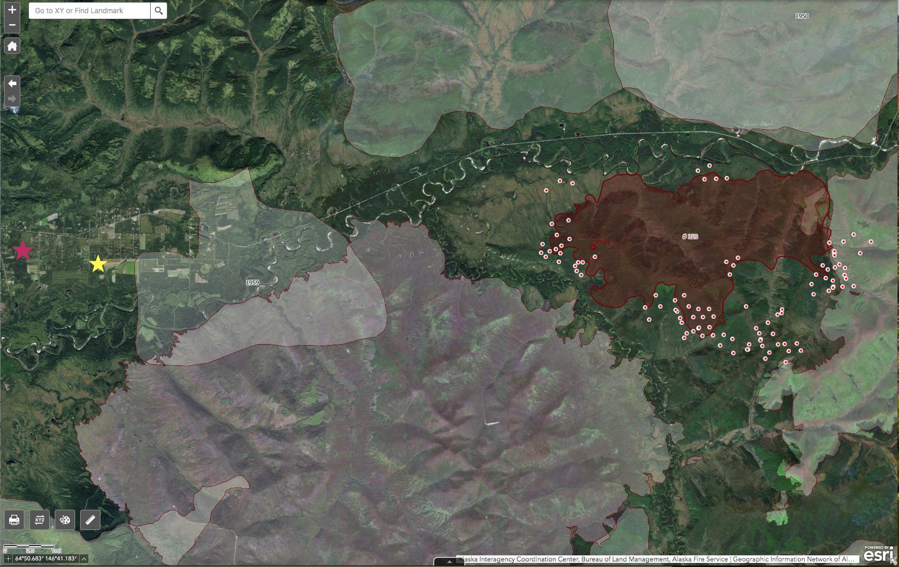
I’m pretty sure that we’ll see some drops of water or retardant if the fire service thinks it may jump over the river or road in the north. There are more reasons to think it won’t spread too far west or east: not only is the western side quite swampy and full of sloughs (and of course a small river), but there are also recent fire scars in the area, which would slow down a fire. The blue area is already within the scar left by the 2013 Stuart Creek 2 fire, and the area east of the fire burned in 2009 or 2000:
Nugget Creek fire as of July 6, with active fire detections around its perimeter. Old fire scars surround the area. The stars indicate where we live, and the location my spouse and I are in the process of moving to. (click for larger image)
So what do I expect will happen? My guess is that the fire will burn out a good part of the triangle between rivers and old fire scars. It’ll be several days before we can expect rain, so smoke will stay terrible for a while.
In any event, Nugget Creek will be an interesting case study for testing models of how fire spreads: It’s one of the few fires that will be relatively easily accessible on foot (once it is completely out of course!), as it has reached Mastodon Creek Trail in the east and is visible from two bridges over the Chena River. And it will have been essentially unsuppressed, ie left ti its natural progression, at least until now.
The vegetation in the Alaskan Interior (roughly the area between two mountain ranges, the Brooks Range in the north and the Alaska Range in the South) mostly consists of boreal forest – black and white spruce, larch, birch and quaking aspen – with easily burnable undergrowth and a thick organic soil layer in the coniferous parts. This type of forest has long been adapted to a cycle driven into a new round by wildfire. But with climate change, the fire intervals – the time between successive burns, usually over 100 years – have become shorter and areas burned have crept upwards.
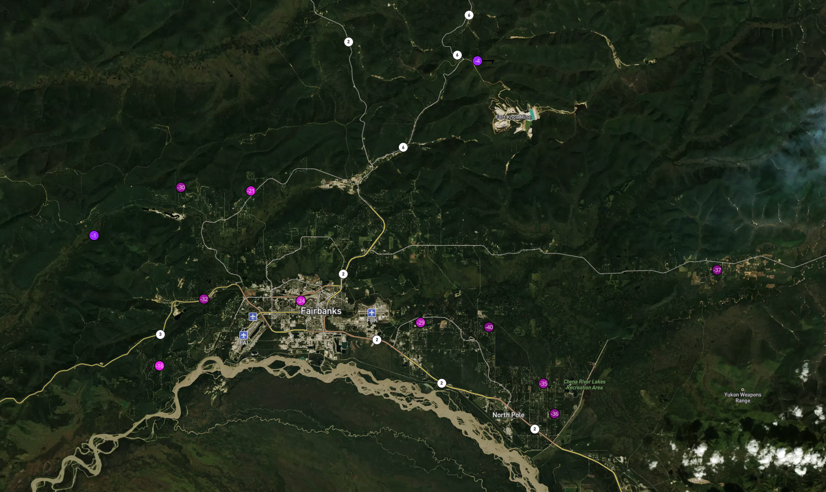
Right now, there are many relatively small fires surrounding Fairbanks that are responsible for the smoke. But they are only kept relatively small by the excellent work of our wildfire management services (a complex effort involving both federal and Alaska state agencies, called Alaska Interagency Coordination Center, or AICC). And one of the fires to the north-west of Fairbanks, the Shovel Creek fire, now exceeds 1000 acres (400 ha), is very active, and has put several residential neighborhoods under an evacuation warning. My partner and I live on the east side of town, and the situation there looks about like this now:
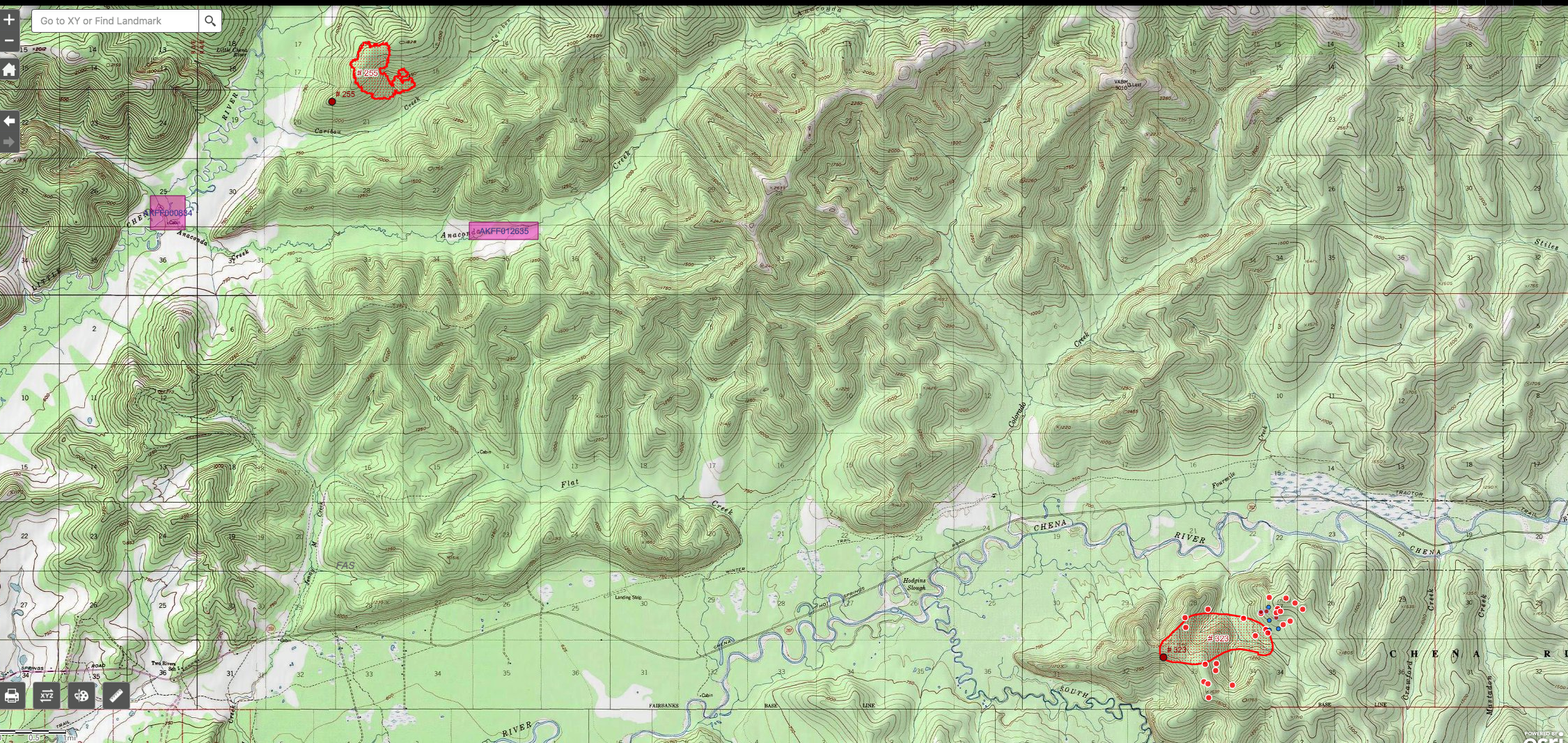
Map of fires as of June 26 (evening) in the area east of Fairbanks. Chena Hot Springs Road, along which most people here live, is along the bottom of the map, partly paralleling the Chena River. Fire perimeter (last known) are the red outlines. Recent fire detections are dots in red (last 12/24 hours) or blue (24-48 hours)
Mapping services and data sources available to the general public have become much more widespread, and that’s great. And private citizens, fire management agencies and researchers publish a wealth of photos. But with the flood information comes a challenge: to learn how to interpret it. Because if we don’t, more information can mean more anxiety. Let’s see how we do for the fires in the area where I live.
Last week, we were mostly worried about the Caribou Creek fire (north edge of the map), which is about 7 miles (11 km) due north of our current home. (My spouse and I are in the process of buying and hopefully soon moving to another home very close by, and the fires are clearly making it harder to get the insurance providers to issue the policies we need!) That fire was immediately strongly attacked, and was already in the process of being controlled after received a good dousing with rain last weekend.
As you can see in the map, there is a fire perimeter as well as one red, black-edged dot that indicates the latitude and longitude where the fire was originally thought to have started. But that’s all. However, for the fire east of us (Nugget Creek fire — many fires here are named after the nearest creek, river or sometimes mountain or street), you can also see white-rimmed red dots as well as blue and darker red dots. These are fire detections from satellite observations, and they are more recent than the fire perimeter drawn by the fire services. So by looking where those dots are relative to the known fire perimeter, you can get an impression where the fire is moving. In this case, mostly east and south, plus a little bit north. (The fire is boxed in by rivers west and further north, luckily.) The reason this fire is more active than Caribou Creek is that it is in an uninhabited area (a state recreation park used by hikers etc.) and was NOT initially fought with vigor. And that’s a good thing in principle: it is normal for this forest to burn occasionally. If we never allow it, dead debris is just going to accumulate, and future fires might be that much worse. However, once the nuisance from the fire becomes too great, or the fire approaches areas where it could do damage, the fire agencies will decide to fight it – which is exactly what happened.
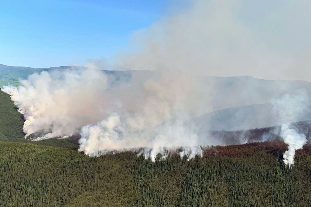
Here are some pictures of the Nugget Creek fire from yesterday that illustrate why concern has risen:
This photo was taken yesterday (Wednesday, June 26) evening by UAF’s Dr. Scott Rupp, from his home north of Chena Hot Springs Road and west of the fire. The Nugget Creek fire is on the left. On the right, the Beaver Fire is a new fire burning further south. Used with permission ( original on Twitter: https://twitter.com/TScottRupp/status/1144089781984305153 ) Photo of the Nugget Creek fire from the same day, Wed. June 26, by the Alaska Department of Natural Resources/Division of Forestry. (Author: Brandon Kobayashi). Looking south as well.
The second photo in particular shows that the fire is active along its perimeter, with the smoke being driven backwards, into the already-burned zone (“fire scar”). This is called “backing”.
Backing is one of the terms for fire behavior that it is useful to know. Even more useful, here in the boreal forest of North America, are “torching” and “spotting”, both considered extreme behaviors Torching is a behavior that happens at high intensities in our spruce forests: individual trees, often one after the next, light up in combustion like a torch, with flames rising high and usually a very large amount of smoke. Spotting is another extreme behavior. It means that the fire is driven forward by wind, jumping ahead of the existing fire front by new ignition from falling embers. The fire in the last picture is a highly active fire, but as of the picture neither torching nor spotting. Especially for spotting, you’d have to have wind that blows in the other direction, driving embers ahead of the front.
Why am I harping on words like “spotting”? Because I’ve been seeing a misconception on social media, created by the excellent new fire maps! Let’s zoom in on the map:
Those dots that signify the locations of new satellite-based fire detections? I’ve seen people on social media call this situation “spotting”. But it is not. In fact, when I make fire maps, I prefer depicting the detection as whole footprints, rectangles (or nearly) that indicate what a satellite image pixel looks on the ground. Because the satellite images we use for this are not high resolution: each dot actually covers an area of about (at least) a quarter mile by a quarter mile.
The hobby linguist in me wonders if, given that the public is now used to these near real-time fire detections being available as dots on a map, maybe the term “spotting” will be more and more used in this way. Because it is relevant whether there are new fire detections or not (though to be honest, that’s a lot more complicated than it looks like at fist). “OMG, there are spots of new fire out to the east… the fire is spotting!” To be sure, if the fire is spotting via flying embers, then it is likely that new detections will show up as dots on the next available map. But I do need to point out that spotting, the extreme fire behavior is not the same as new spots on a map. Rather, any movement of the fire, even medium-intensity propagation of the combustion with no spotting at all, will appear as new dots. “Spotting” means a particular way of a high-intensity fire moving ahead, and new fire detections on a map are just new fire detections on a map.
Sources of fire information for Alaska:
AK Fire Info. Blog-style, up to date, excellent information about what’s going on, which fires receive what type of attention, planned community meetings, pictures and more.
Official BLM/AICC map site. Tip: Use the icons to select the background you like. I prefer “US Topo Map” or “Imagery with labels”.
“Old” BLM/AICC map site – harder to navigate, but has also some information the new one hasn’t.
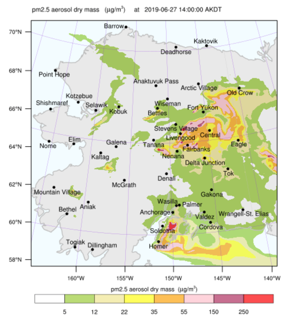
UAF Smoke forecasts, run daily based on satellite fire detections and AICC data. Also has a simple “current fires” map.
NOAA smoke forecasts for Alaska. May be interesting for people in the Yukon Territory in Canada. Click on the check mark between “near surface smoke” and “loop”.
After an incredibly warm (and low-snow) start of winter in 2018, temperatures plunged to proper sub-Arctic winter values. A few days ago, we were worrying about thawing (with temperatures in the 30s °F / around 0 °C), and then down the curve went. Last night we reached -40 (choose your unit: the scales meet at -40) as per our consumer-grade Davis weather station. That’s the official definition of “cold snap”, and it’s the first of the season.
Higher elevations, such as Cleary Summit, a mountain pass on the Steese Highway north of Fairbanks, are currently about 30 °F/17 °C warmer than the valley bottoms. Where we happen to live (and which is why “a house in the hills” is something we keep looking out for).
Life as -40 slows down. You can go out just fine, and you’ll be amazed by how well sled dogs are adapted to this extremely harsh weather, but it’s not really fun to exercise outside, plastic is brittle, batteries go flat … and you don’t have time for recreation because you need to keep an eye on the house systems. Especially to make sure that water stays liquid, be it in drains or incoming pipes.
The house we live in is made from three-sided logs, which retain heat quite well. We mostly heat with a very efficient and Toyo oil stove. But we have a wood stove to fall back on, in case the electricity or the Toyo have an outage. We decided to fire it up today, to make sure it works well and because it creates a nicer warmth in the corners too far from the Toyo. Wood burning is a huge and complicated political hot potato in interior Alaska, and a topic too complicated to go into in this post. The short version is: it’s traditional, economical and doesn’t require electricity; but it also contributes to air pollution in a way to occasionally render the winter air in Fairbanks one of the worst in the planet, so at a minimum eliminating the most polluting types of burners is quite imperative for the health of the population.
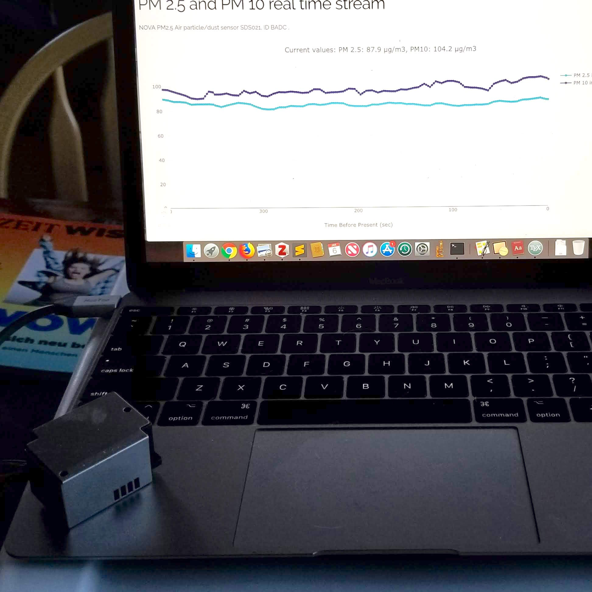
Our stove is an EPA-certified Blaze King with a catalytic converter, but even so: however pleasant wood heat is, you’ll get an impact on the air you breathe. Air quality indices only talk about outdoors air (and usually averaged over 24h). Another topic, though, is indoors air. I took the opportunity to pull out a little PM2.5 sensor that I bought online a while ago. (Disclaimer: I haven’t checked the calibration. At least during the summer wildfires it seemed to work reasonably well and deliver believable values.) Today, before starting the wood stove and with a blazing oil stove, it measured around 15 µg/m3, which is an ok value. With the wood stove, it was at 66 µg/m3 after an hour, went up to just above 100 µg/m3 and then settled in the 80s, which you will find labeled as “unhealthy for vulnerable populations”. My setup is here, with the sensor in the left foreground. It talks to the computer via a USB-to-serial interface. (I wrote the app to teach myself Dash for interactive real-time applications.)
This, of course, is measured indoors, not outdoors, and in the 24h average we will quite likely end up in the “moderate” range for the day. We’re fine.
On a related note, no one should retain too rosy a picture of the air pre-historic and pre-industrial populations used to breathe. Notwithstanding, of course, their insights about the relationship to nature: if a culture or people practices indoors wood or coal burning for cooking and warmth, chances are that respiratory illnesses were prevalent.
Addendum: Approximately 5-6 h after we first started the wood stove, the picture has changed a little bit. PM2.5 values came progressively down to 15-25 µg/m3, pretty much to where they were before we started. Clearly, the first fire-up phase is what generates the most pollution, while collected crud from inside and outside the stove burned off. In contrast, low-to-medium hot, steady operation deteriorates the air much less. Also, I believe it takes a few hours for the catalytic converter to reach its operating temperature. Apparently, letting the stove cool down completely and sit cold for extended periods is a recipe for air pollution. The lesson from this is: If you want to heat with firewood, make sure you have a device with a certified catalytic converter, use it continuously and burn dry, well-seasoned wood.
I called it a shootout first, but hey, it wasn’t anything violent.
Sensing temperature with Python and the pyboard
Because I have the best spouse in the world, my recent birthday brought me a whole pile of little boxes with electronic tinker toys, useful ones, straight from Hackerboxes. I’ve since been renewing my acquaintance with the soldering iron and dusted off an old project about building environmental sensor units.
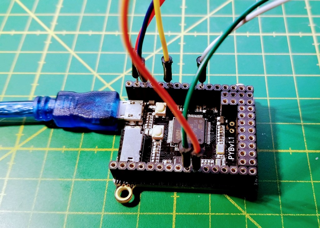
One of the development boards I was keen to try out is the pyboard, which is the original or official board for MicroPython. MicroPython is a new implementation of a remarkably rich subset of Python 3.4 to run on microprocessors. I already had a good deal of experience with CircuitPython, the education-friendly derivative of MicroPython published and maintained by Adafruit. Now it was time for the real thing.
The pyboard is very compact. For comparison, the grid on my work surface are 1×1 cm.
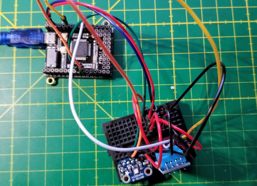
So the plan I came up with is: Gather the temperature sensors from my kit, hook them all up to the pyboard at the same time, log the temperature for a while and compare the outcome.
The sensors
After rummaging through my component boxes, I fished out these three sensors (pictures below):
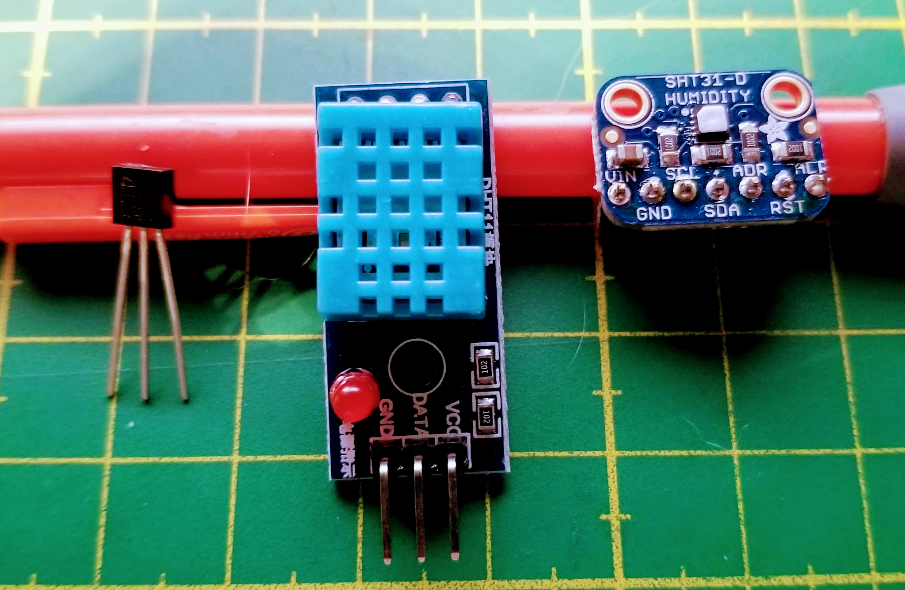
The TMP36 is a popular low-cost silicon band gap temperature sensor. It is small, with three output pins, and comes in a black plastic housing. T range: -40-150 °C, T accuracy ±2 °C. Price: $ 1.50
The DHT11 is a very common temperature and relative humidity sensor with not the best reputation for accuracy. It comes in a blue housing with electronic components included, and our version (from a Hackerbox) is mounted onto a small board, which adds a pull-up resistor and a power LED. The DHT11 documentation is a little spotty. The sensor apparently uses a negative temperature coefficient (NTC) thermistor (ie, temperature goes up → resistance goes down) and some kind of resistive humidity measurement. The sensor can only take T measurements every 2 sec. T range: 0-50 °C, T accuracy ±2 °C, RH accuracy ± 5%. Price: $ 5
The most expensive item in this set, the Sensiron SHT31-D, uses a CMOS chip to measure temperature and relative humidity, with a capacitive method. I used the lovely little Adafruit breakout board. T range: -40-125 °C, T accuracy ±0.3 °C (between 0 and 60 °C) and up to ±1.3 °C at the edges, RH accuracy ± 2%. Price: $ 14.
The prices are 2018 prices from US vendors. By ordering directly from Chinese outlets, you can usually reduce them to ~40%, except for the much rarer SHT31-D, for which only one ready-to-use alternative (which is not much cheaper) appears to exist.
The three temperature sensors: TMP36 (left), DHT11 (middle), SHT31-D (right).The whole setup.
Two related consideration at this stage: What communication protocol do the sensors use, and what MicroPython libraries are available to drive them from the pyboard?
While the documentation for MicroPython is superb, I found the pyboard to be a lot less well documented. MicroPython comes with a library specific to the pyboard (pyb) as well as generic libraries that are supposed to work with any supported board (eg. machine), and their functions sometimes overlap. I had to consult the MicroPython forum a few times to figure out the best approach.
The TMP36 is a single-channel analog sensor: The output voltage is linear in the temperature (it boasts a linearity of better than 0.5%). So we need a DAC pin to measure the output voltage at the pyboard (using a DAC object from the pyb module). According to a forum post, the pin output is a 12-bit integer (0-4095) that is proportional to the voltage (0-3.3V). So we get the voltage in mV by multiplying the pin value by 3300 and dividing by 4095. Then, as per the TMP36 datasheet, we have to subtract 500 and divide by 10 to convert that value to °C. Easy.
The DHT11 also uses single channel protocol, but a digital one, which looks a little idiosyncratic. (I was a little surprised to find that none of my sensors uses the popular 1-Wire bus.) Luckily, MicroPython ships with a library (dht) that takes care of everything. It outputs temperature in °C and relative humidity in %.
I was particularly happy how easy it is to scan the I2C bus for the device port with MicroPython. From the MicroPython REPL (which you enter to as soon as you connect to a new pyboard via a terminal emulator like screen), it’s great to be able to create and probe objects interactively, for example like so:
This said, the sht31 library doesn’t even need the user to provide the port. I’m just noting this because this task can be a little frustrating on the Arduino platform, and take more tries to get it done.
Our basic workflow was this:
Using the MicroPython REPL, develop the MicroPython code incrementally. The goal is to take a measurement every 10 sec and send the data back to the computer over the USB serial port.
I let the experiment run for a few overnight hours in my somewhat overheated home office corner, where the air is very dry.
The measurement results
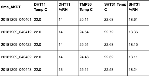
Even while monitoring the data flow, some observations stand out: The DHT11 only provides temperatures in whole degrees. And the temperature measured with the TMP36 is a good bit (about 2-3 °C) higher than the output from the other two sensors. The data looks somewhat like this:
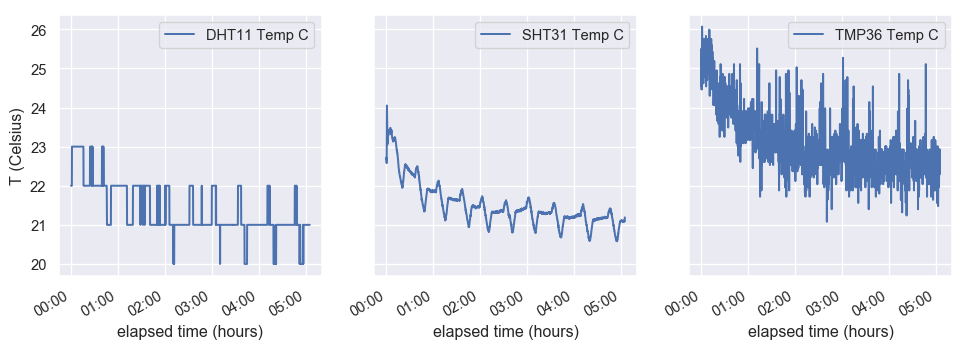
Let’s look at plots of the three temperature curves. At first, I was not impressed: The DHT11 measurements seemed to jump around a whole lot, the SHT31 has a very weird periodic signal and the TMP36 data is incredibly noisy (apart from unrealistically high – the room wasn’t that badly overheated!).
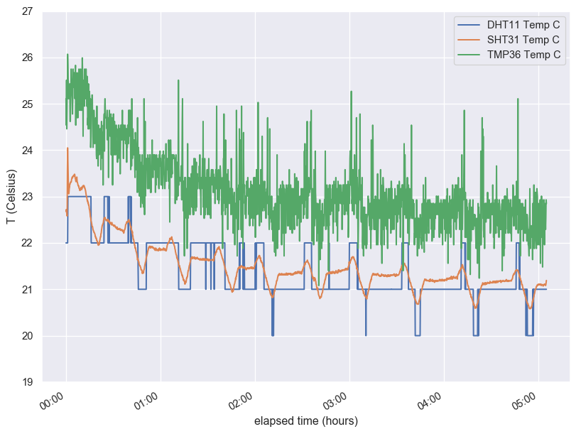
But things become clearer once we plot onto a single figure: The upticks of the DHT11 measurement correspond exactly to the peaks of the SHT31 data, and so do the minima! Also, the two sensors agree, within their precision, quite well in absolute value. Once I took the SHT31 signal seriously, I realized what it was due to: The thermostat cycle of our Toyo oil stove! I had no idea that it was on this 30 min cycle. How interesting. And now that I know, I really like the SHT31. (Apparently you get what you pay for in this case.)
What about the TMP36? Well, it’s noisy and operating way outside its nominal accuracy, but at least some of the signal is clearly due to the real temperature variation.
The fall-off of the data during the first hour is, btw, probably because I removed my body from the desk and went to bed. The air cooled afterwards.
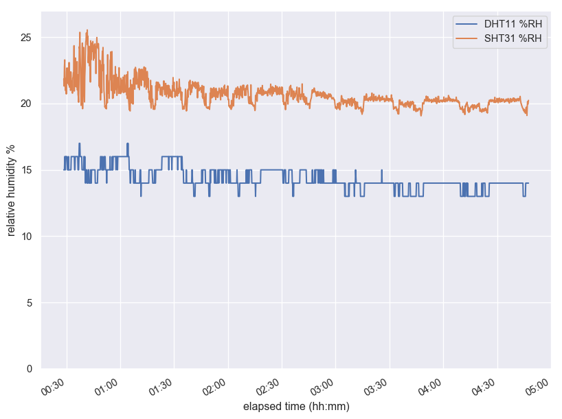
Since I had the relative humidity data, I looked at it, too. Here the SHT31 and the DHT11 agree less well in absolute value, and I think the latter is in agreement with its reputation as not very accurate. I find the SHT31 values a lot more convincing. One thing that the graphs don’t show is that if you blow on the sensor, the SHT31 adjusts immediately and goes back to normal pretty fast, while the DHT11 takes a few seconds for its measurement to jump. It also saturates quickly (showing unrealistic nearly-100% of RH) and takes a long time to return from an extreme measurement.
What did we learn? What else could we find out?
So this was interesting! I didn’t expect to get so clear a feeling for the different sensors’ strengths and weaknesses. At the same time, I’m have more questions…
The DHT11 confirmed its reputation as a very basic sensor. Its temperature measurement was in better agreement with what I think is reality than expected, but the relative humidity is not very trustworthy. Its limited range and whole-degree step size make it a mediocre choice for a personal weather station, and its slowness unsuitable for, say, monitoring temperature sensitive circuitry. But could we get a higher resolution with a different software library? Are there settings that escaped my notice? As-is, I see its application mostly in education and maybe indoors monitoring when you don’t need much precision.
The TMP36 was disappointing, but maybe my expectations of this $ 1.50 sensor were excessively high. As an analog sensor, it is faster than the DHT11 (though I don’t know how fast … just yet) and can be used for monitoring temperature extremes, but not with high precision because of the noise! Maybe a good approach would be to reduce the noise in some fashion. Also, did I have a bum unit, or do they all need calibrating? Maybe the pyboard-specific conversion formula has a flaw, and a different board or method would produce a different result?
The SHT31-D looks like a great sensor all around. Also congratulations to Adafruit for producing an outstanding breakout board. This would be my choice for a weather station, hands down.
Other questions I have are: How different would the performance be in a different temperature range? I live in Alaska, and temps went down to -30 °C today. (My medium-term plan is to put a sensor under the snow.) Also, how fast can we actually retrieve successive measurements from our two faster sensors? Last, I think I found at least two more temperature sensors in my kit. How do they compare?