The great temperature sensor tryout (part 1)

I called it a shootout first, but hey, it wasn’t anything violent.

Sensing temperature with Python and the pyboard

Because I have the best spouse in the world, my recent birthday brought me a whole pile of little boxes with electronic tinker toys, useful ones, straight from Hackerboxes. I’ve since been renewing my acquaintance with the soldering iron and dusted off an old project about building environmental sensor units.

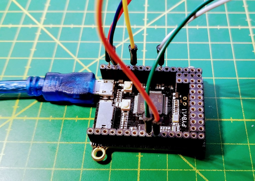
One of the development boards I was keen to try out is the pyboard, which is the original or official board for MicroPython. MicroPython is a new implementation of a remarkably rich subset of Python 3.4 to run on microprocessors. I already had a good deal of experience with CircuitPython, the education-friendly derivative of MicroPython published and maintained by Adafruit. Now it was time for the real thing.

The pyboard is very compact. For comparison, the grid on my work surface are 1×1 cm.

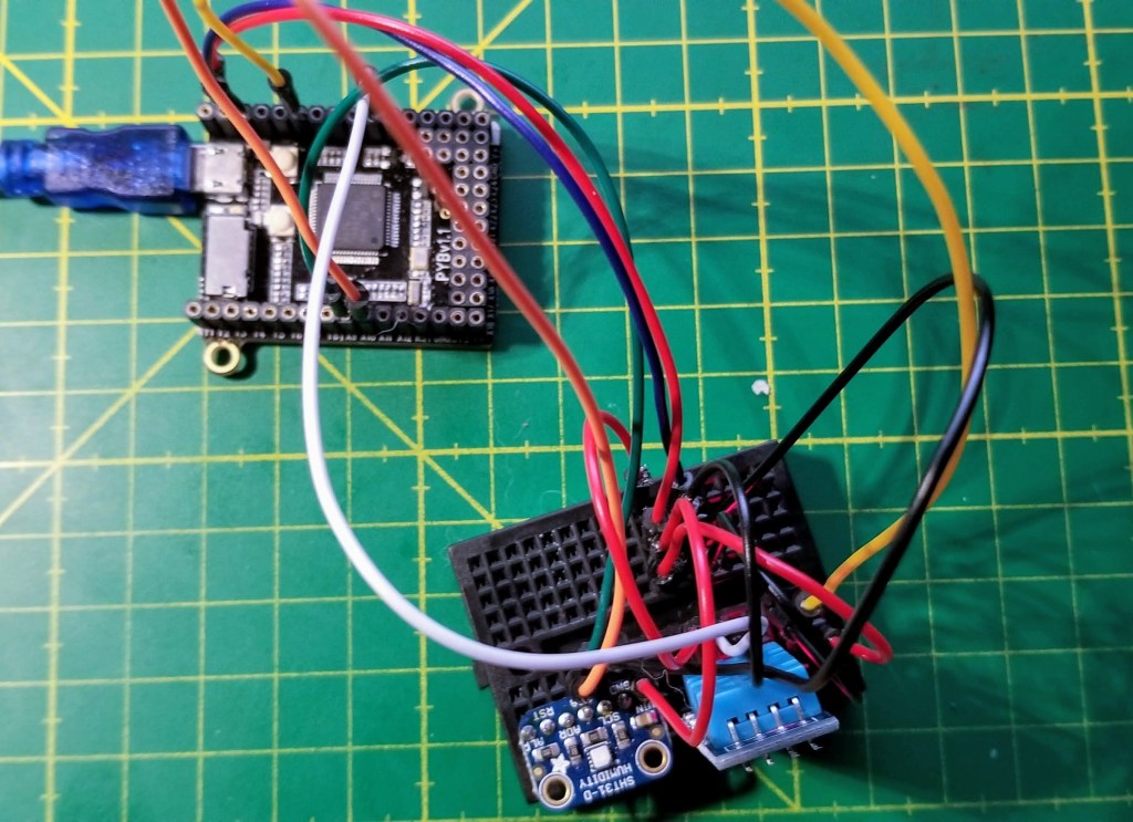
So the plan I came up with is: Gather the temperature sensors from my kit, hook them all up to the pyboard at the same time, log the temperature for a while and compare the outcome.

The sensors

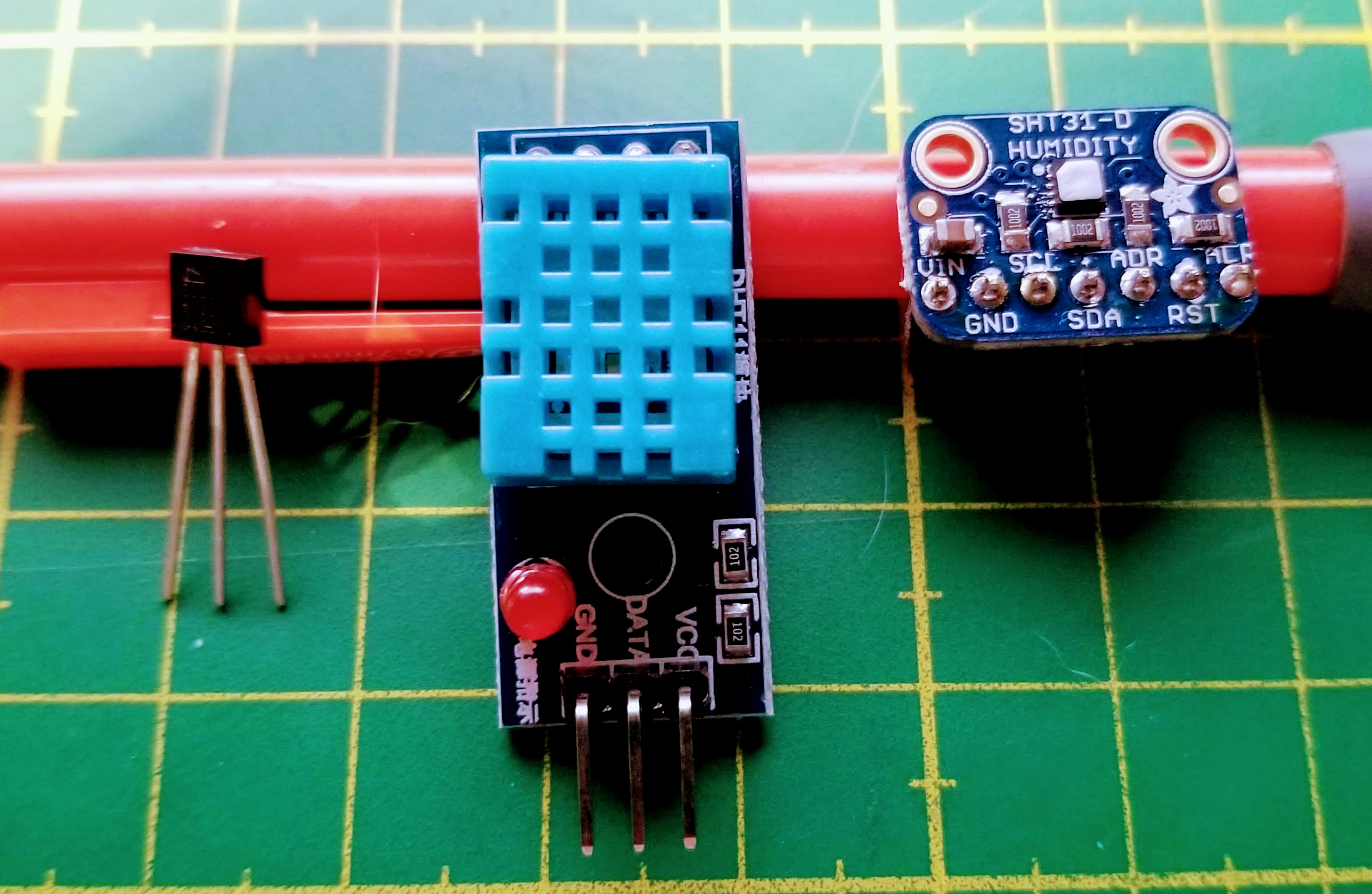
After rummaging through my component boxes, I fished out these three sensors (pictures below):

The TMP36 is a popular low-cost silicon band gap temperature sensor. It is small, with three output pins, and comes in a black plastic housing. T range: -40-150 °C, T accuracy ±2 °C. Price: $ 1.50
The DHT11 is a very common temperature and relative humidity sensor with not the best reputation for accuracy. It comes in a blue housing with electronic components included, and our version (from a Hackerbox) is mounted onto a small board, which adds a pull-up resistor and a power LED. The DHT11 documentation is a little spotty. The sensor apparently uses a negative temperature coefficient (NTC) thermistor (ie, temperature goes up → resistance goes down) and some kind of resistive humidity measurement. The sensor can only take T measurements every 2 sec. T range: 0-50 °C, T accuracy ±2 °C, RH accuracy ± 5%. Price: $ 5
The most expensive item in this set, the Sensiron SHT31-D, uses a CMOS chip to measure temperature and relative humidity, with a capacitive method. I used the lovely little Adafruit breakout board. T range: -40-125 °C, T accuracy ±0.3 °C (between 0 and 60 °C) and up to ±1.3 °C at the edges, RH accuracy ± 2%. Price: $ 14.

The prices are 2018 prices from US vendors. By ordering directly from Chinese outlets, you can usually reduce them to ~40%, except for the much rarer SHT31-D, for which only one ready-to-use alternative (which is not much cheaper) appears to exist.

The three temperature sensors: TMP36 (left), DHT11 (middle), SHT31-D (right).

Communication protocols, libraries, and code

All code, both on the computer side and the pyboard side, is available in a git repository on GitHub.

Two related consideration at this stage: What communication protocol do the sensors use, and what MicroPython libraries are available to drive them from the pyboard?

While the documentation for MicroPython is superb, I found the pyboard to be a lot less well documented. MicroPython comes with a library specific to the pyboard (pyb) as well as generic libraries that are supposed to work with any supported board (eg. machine), and their functions sometimes overlap. I had to consult the MicroPython forum a few times to figure out the best approach.

The TMP36 is a single-channel analog sensor: The output voltage is linear in the temperature (it boasts a linearity of better than 0.5%). So we need a DAC pin to measure the output voltage at the pyboard (using a DAC object from the pyb module). According to a forum post, the pin output is a 12-bit integer (0-4095) that is proportional to the voltage (0-3.3V). So we get the voltage in mV by multiplying the pin value by 3300 and dividing by 4095. Then, as per the TMP36 datasheet, we have to subtract 500 and divide by 10 to convert that value to °C. Easy.
The DHT11 also uses single channel protocol, but a digital one, which looks a little idiosyncratic. (I was a little surprised to find that none of my sensors uses the popular 1-Wire bus.) Luckily, MicroPython ships with a library (dht) that takes care of everything. It outputs temperature in °C and relative humidity in %.
The SHT31-D communicates via an I2C bus. I used MicroPython’s generic machine module and sht31 module provided by kfricke that builds on it.

I was particularly happy how easy it is to scan the I2C bus for the device port with MicroPython. From the MicroPython REPL (which you enter to as soon as you connect to a new pyboard via a terminal emulator like screen), it’s great to be able to create and probe objects interactively, for example like so:

>> import machine
>> SCLpin = 'X9'
>> SDApin = 'X10'
>> i2c = machine.I2C(sda=machine.Pin(SDApin), 
                     scl=machine.Pin(SCLpin), 
                     freq=400000)
>> i2c.scan()

This said, the sht31 library doesn’t even need the user to provide the port. I’m just noting this because this task can be a little frustrating on the Arduino platform, and take more tries to get it done.

Our basic workflow was this:

Using the MicroPython REPL, develop the MicroPython code incrementally. The goal is to take a measurement every 10 sec and send the data back to the computer over the USB serial port.
Upload finished MicroPython code to the pyboard.
Use the USB connection now to receive serial data from the pyboard (using Python 3 on the computer) and also to power the board.
Let the assembly collect data for a few hours and write it to a file.
Visualize the data afterwards.

I let the experiment run for a few overnight hours in my somewhat overheated home office corner, where the air is very dry.

The measurement results

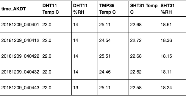
Even while monitoring the data flow, some observations stand out: The DHT11 only provides temperatures in whole degrees. And the temperature measured with the TMP36 is a good bit (about 2-3 °C) higher than the output from the other two sensors. The data looks somewhat like this:

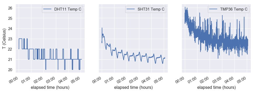
Let’s look at plots of the three temperature curves. At first, I was not impressed: The DHT11 measurements seemed to jump around a whole lot, the SHT31 has a very weird periodic signal and the TMP36 data is incredibly noisy (apart from unrealistically high – the room wasn’t that badly overheated!).

But things become clearer once we plot onto a single figure: The upticks of the DHT11 measurement correspond exactly to the peaks of the SHT31 data, and so do the minima! Also, the two sensors agree, within their precision, quite well in absolute value. Once I took the SHT31 signal seriously, I realized what it was due to: The thermostat cycle of our Toyo oil stove! I had no idea that it was on this 30 min cycle. How interesting. And now that I know, I really like the SHT31. (Apparently you get what you pay for in this case.)

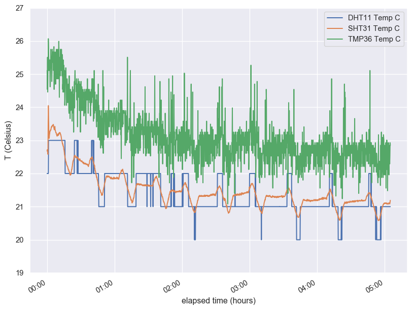
What about the TMP36? Well, it’s noisy and operating way outside its nominal accuracy, but at least some of the signal is clearly due to the real temperature variation.

The fall-off of the data during the first hour is, btw, probably because I removed my body from the desk and went to bed. The air cooled afterwards.

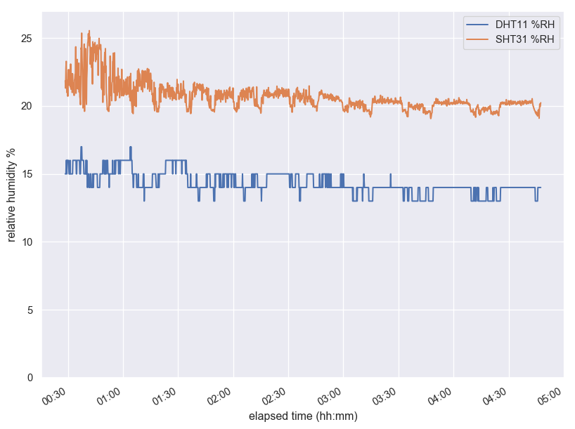
Since I had the relative humidity data, I looked at it, too. Here the SHT31 and the DHT11 agree less well in absolute value, and I think the latter is in agreement with its reputation as not very accurate. I find the SHT31 values a lot more convincing. One thing that the graphs don’t show is that if you blow on the sensor, the SHT31 adjusts immediately and goes back to normal pretty fast, while the DHT11 takes a few seconds for its measurement to jump. It also saturates quickly (showing unrealistic nearly-100% of RH) and takes a long time to return from an extreme measurement.

What did we learn? What else could we find out?

So this was interesting! I didn’t expect to get so clear a feeling for the different sensors’ strengths and weaknesses. At the same time, I’m have more questions…

The DHT11 confirmed its reputation as a very basic sensor. Its temperature measurement was in better agreement with what I think is reality than expected, but the relative humidity is not very trustworthy. Its limited range and whole-degree step size make it a mediocre choice for a personal weather station, and its slowness unsuitable for, say, monitoring temperature sensitive circuitry. But could we get a higher resolution with a different software library? Are there settings that escaped my notice? As-is, I see its application mostly in education and maybe indoors monitoring when you don’t need much precision.
The TMP36 was disappointing, but maybe my expectations of this $ 1.50 sensor were excessively high. As an analog sensor, it is faster than the DHT11 (though I don’t know how fast … just yet) and can be used for monitoring temperature extremes, but not with high precision because of the noise! Maybe a good approach would be to reduce the noise in some fashion. Also, did I have a bum unit, or do they all need calibrating? Maybe the pyboard-specific conversion formula has a flaw, and a different board or method would produce a different result?
The SHT31-D looks like a great sensor all around. Also congratulations to Adafruit for producing an outstanding breakout board. This would be my choice for a weather station, hands down.

Other questions I have are: How different would the performance be in a different temperature range? I live in Alaska, and temps went down to -30 °C today. (My medium-term plan is to put a sensor under the snow.) Also, how fast can we actually retrieve successive measurements from our two faster sensors? Last, I think I found at least two more temperature sensors in my kit. How do they compare?

I think there might be a part 2 in the works…

Plotting polygon Shapefiles on a Matplotlib Basemap with GeoPandas, Shapely and Descartes

I often use Python to plot data on a map and like to use the Matplotlib Basemap Toolkit. In practice, I use a lot of different libraries to access various data formats (raster, vector, serialized…), select and analyse them, generate, save and visualize outputs, and it’s not always obvious to string one’s favourite tools together into efficient processing chains.

For example, I’ve also become fond of Pandas DataFrames, which offer a great interface to statistical analysis (e.g. the statsmodels module), and its geo-enabled version, GeoPandas. Both Basemap and GeoPandas can deal with the popular (alas!) ESRI Shapefile format, which is what many many (vector) GIS datasets are published in. But they aren’t made for working together. This post is about how I currently go about processing Shapefile data with GeoPandas first and then plotting it on a map using Basemap. I’m using an extremely simple example: a polygon Shapefile of the earth’s glaciated areas from the handy, and free, NaturalEarth Data site. The data is already in geographic coordinates (latitudes/longitudes), with a WGS 84 datum. We therefore don’t have to worry about preprocessing the input with suitable coordinate transforms. (Often, you do have to think about this sort of thing before you get going…). All my code is available in an IPython (or Jupyther) Notebook, which should work with both Python 2 and 3.

So let’s say we have our glacier data in a file called ne_10m_glaciated_areas.shp. GeoPandas can read this file directly:

import geopandas as gp
glaciers = gp.GeoDataFrame.from_file(
    'ne_10m_glaciated_areas/ne_10m_glaciated_areas.shp')
glaciers.head()

The output looks something like this:

Screen Shot 2016-03-06 at 17.02.23

The geometry column (a GeoSeries) contains Shapely geometries, which is very convenient for further processing. These are either of type Polygon, or MultiPolygon for glaciers with multiple disjoint parts. GeoPandas GeoDataFrames or GeoSeries can be visualized extremely easily. However, for large global datasets, the result may be disappointing:

glaciers.plot()

allglaciers

If we want to focus on a small area of the earth, we have a number of options: we can use Matplotlib to set the x- and y-limits of the plot. Or we can filter the dataset geographically, and only, say, plot those glaciers that intersect a rectangular area in the vicinity of Juneau, AK, that is, the Alaskan Panhandle and the adjacent Western British Columbia. Filtering the dataset first also speeds up plotting, by a lot:

import shapely
studyarea = shapely.geometry.box(-136., 56., -130., 60.)
ax1 = glaciers[glaciers.geometry.intersects(studyarea)].plot()
ax1.set_aspect(2)
fig = plt.gcf()
fig.set_size_inches(10, 10)

glaciersselect

This is remarkable for so few lines of code, but it’s also as far as as we can get with GeoPandas alone. For more sophisticated maps, enter Basemap. The Basemap module offers two major tools:

a Basemap class that represents a map in a pretty good selection of coordinate systems and is able to transform arbitrary (longitude, latitude) coordinate pairs into the map’s coordinates
a rich database of country and state borders, water bodies, coast lines, all in multiple spatial resolutions

Features that add on to these include plotting parallels and meridians, scale bars, and reading Shapefiles. But we don’t want to use Basemap to read our Shapefile — we want to plot the selections we’ve already made from the Shapefile on top of it.

The basic syntax is to instantiate a Basemap with whatever options one finds suitable:

mm = Basemap(projection=..., width=..., height=...)

… and then to add whatever other features we want. To transform a (longitude, latitude) coordinate pair, we use mm(lon, lat). The resulting transformed coordinates can then be plotted on the map the usual Matplotlib way, for example via mm.scatter(x, y, size, ...). The code to plot our study area and the city of Juneau, in the Albers Equal Area conical projection (good for high- and low-latitude regions), at intermediate resolution, and including water, ocean, coastlines, country borders etc. is:

from mpl_toolkits.basemap import Basemap
import numpy as np
water = 'lightskyblue'
earth = 'cornsilk'
juneau_lon, juneau_lat = -134.4167, 58.3

fig, ax1 = plt.subplots(figsize=(12, 10))
mm = Basemap(
    width=600000, height=400000,
    resolution='i',
    projection='aea',
    ellps='WGS84',
    lat_1=55., lat_2=65.,
    lat_0=58., lon_0=-134)
coast = mm.drawcoastlines()
rivers = mm.drawrivers(color=water, linewidth=1.5)
continents = mm.fillcontinents(
    color=earth,
    lake_color=water)
bound= mm.drawmapboundary(fill_color=water)
countries = mm.drawcountries()
merid = mm.drawmeridians(
    np.arange(-180, 180, 2), 
    labels=[False, False, False, True])
parall = mm.drawparallels(
    np.arange(0, 80), 
    labels=[True, True, False, False])
x, y = mm(juneau_lon, juneau_lat)
juneau = mm.scatter(x, y, 80, 
    label=&quot;Juneau&quot;, color='red', zorder=10)

juneaumap

This result may even be quite suitable for publication-quality maps. To add our polygons, we need two more ingredients:

shapely.ops.transform is a function that applies a coordinate transformation (that is, a function that operates on coordinate pairs) to whole Shapely geometries
The Descartes library provides a PolygonPatch object suitable to be added to a Matplotlib plot

To put it together, we need to take into account the difference between Polygon and MultiPolygon types:

patches = []
selection = glaciers[glaciers.geometry.intersects(studyarea)]
for poly in selection.geometry:
    if poly.geom_type == 'Polygon':
        mpoly = shapely.ops.transform(mm, poly)
        patches.append(PolygonPatch(mpoly))
    elif poly.geom_type == 'MultiPolygon':
        for subpoly in poly:
            mpoly = shapely.ops.transform(mm, poly)
            patches.append(PolygonPatch(mpoly))
    else:
        print(poly, &quot;is neither a polygon nor a multi-polygon. Skipping it.&quot;)
glaciers = ax1.add_collection(
    PatchCollection(patches, match_original=True))

The final result, now in high resolution, looks like this:

glaciersmap
We could do a lot more — add labels, plot glaciers in different colors, for example. Feel free to play with the code.

Data type mapping when using Python/GDAL to write Numpy arrays to GeoTIFF

Numpy arrays are a fundamental tool for scientific data processing in Python. To deal with spatial data that is geo-referenced on a rectangular-grid raster the GeoTIFF file format is similarly ubiquitous. Saving spatial data that is held in a Numpy array to a GeoTIFF file should therefore be an extremely common task, so it was surprising to me to run into some pitfalls. This post is a write-up on how to get around them.

To access GeoTIFF files I’m using the Geospatial Data Abstraction Library (GDAL), a powerful set of tools that comes with multiple command line utilities and bindings for the most common scripting languages used in science. As it is originally a C/C++ library, it can be quite unpythonic — one of many reasons why you might want to write your own library for your specific purpose.

Writing a Numpy array to a GeoTIFF file consists of these steps:

Figure out the spatial reference system (coordinate system and, if applicable, map projection), usually from the source data set, and get the Well-Known Text representation of it (examples).
Figure out the geotransform, that is the parameters that describe how the data has to be shifted and stretched to place it on the spatial reference system. This, too, will be derived from the source data and whatever manipulations were subsequently carried out.
Create a dataset object using GDAL’s “GTiff” driver, attach the spatial reference and geotransform, and write out the data

The details are described in the GDAL API tutorial and elsewhere on the web. In the simplest case, if the data originates from another GeoTIFF file, has only one raster band, and we didn’t sub-set or re-scale it (geographically), we could do this [1]:

from osgeo import gdal

src_dataset = gdal.Open("[input GeoTIFF file path]")
src_data = src_dataset.ReadAsArray()
# final_data is a 2-D Numpy array of the same dimensions as src_data
final_data = some_complicated_scientific_stuff(src_data, other_data, ...)

# get parameters
geotransform = src_dataset.GetGeoTransform()
spatialreference = src_dataset.GetProjection()
ncol = src_dataset.RasterXSize
nrow = src_dataset.RasterYSize
nband = 1

# create dataset for output
fmt = 'GTiff'
driver = gdal.GetDriverByName(fmt)
dst_dataset = driver.Create([output_filepath], ncol, nrow, nband, gdal.GDT_Byte)
dst_dataset.SetGeoTransform(geotransform)
dst_dataset.SetProjection(spatialreference)
dst_dataset.GetRasterBand(1).WriteArray(final_data)
dst_dataset = None

Thus far, there’s nothing difficult about it. But the problem arises on line 18, where the data type is passed to the Create() method. gdal.GDT_Byte refers to a code for GDAL’s Byte data type, that is, an 8-bit unsigned integer. If the final data is of a different type, 16-byte signed integers, say, or floating-point numbers, I could use one of the other GDAL data types.

But I’m writing a library and am therefore unlikely to know the data type beforehand. So what is needed is a general mapping from Numpy dtype objects to GDALDataType objects. And that problem had me stumped for a moment.

OK, it would be possible to guess — there aren’t that many of them — but shouldn’t there be a function?

I found out that in the gdal_array module, there is a function called NumericTypeCodeToGDALTypeCode, which is supposed to translate a “numeric” type into a GDAL type code, for example:

>>> print(gdal_array.NumericTypeCodeToGDALTypeCode(numpy.float32))
6

But it turns out that passing in the dtype attribute of a Numpy array doesn’t work:

>>> print(gdal_array.NumericTypeCodeToGDALTypeCode(my_data.dtype))
...
TypeError: Input must be a type

Nonetheless:

>>> my_data.dtype == numpy.float32
True

Huh? Well, the first thing I learnt from the Python documentation is that for the == operator to return True the two objects aren’t always required to have the same type. In some cases this seems to make more sense than in others.

The second is that evidently, gdal_array.NumericTypeCodeToGDALTypeCode expects an object of type type (that is, Python type), which numpy.float32 appears to be, whereas my_data.dtype is, surprise surprise of type numpy.dtype.

Apparently, the GDAL developers have recognized this behavior as a bug and fixed it in v. 2.0. What can we do meanwhile? The answer, from a StackOverflow post, is that we can instantiate a list of arrays of length 1 that cover all possible Nympy data types and then use numpy.asscalar to convert them to native Python objects with native Python types. For example:

import numpy as np
from osgeo import gdal, gdal_array

typemap = {}
for name in dir(np):
    obj = getattr(np, name)
    if hasattr(obj, 'dtype'):
        try:
            npn = obj(0)
            nat = np.asscalar(npn)
            if gdal_array.NumericTypeCodeToGDALTypeCode(npn.dtype.type):
                typemap[npn.dtype.name] = gdal_array.NumericTypeCodeToGDALTypeCode(npn.dtype.type)
        except:
            pass

(If we want the GDAL Data Type labels, we can use gdal.GetDataTypeName(typecodeinteger).)

This generates a conversion dictionary that looks like this:

NP2GDAL_CONVERSION = {
  "uint8": 1,
  "int8": 1,
  "uint16": 2,
  "int16": 3,
  "uint32": 4,
  "int32": 5,
  "float32": 6,
  "float64": 7,
  "complex64": 10,
  "complex128": 11,
}

(If we want the GDAL Data Type labels, we can use gdal.GetDataTypeName(typecodeinteger).)

That’s a start. Some hand-editing is in order, for example, mapping Booleans to 1 to make it possible to encode them as integers for persistence — clearly, GDAL has no notion of bit or binary objects. Also, it is odd that both int8 and uint8 should be mapped to GDAL Byte types, that is, unsigned integers. That needs to be taken into account when manipulating the data. In addition, several complex Numpy datatypes are missing and could be manually mapped to 10 or 11.

But I can work with this. To get back to the first listing, in the “get parameters” section I add a line and then create the destination dataset as follows:

gdaltype = NP2GDAL_CONVERSION[final_data.dtype.name]
[...]
dst_dataset = driver.Create([output_filepath], ncol, nrow, nband, gdaltype)

Voilà.

NOTES:

[1] I am aware I could have used CreateCopy() in such a simple case, but Create() is more generally versatile.

The second note is that I am aware that the problem isn’t specific to GeoTIFF files: it arises for any data file with GDAL whose driver supports a Create() method. But to be honest, GDAL is pretty unwieldy for most scientific data formats, so if I were to write NetCDF or HDF5 files, I would use appropriate specific libraries, most of which tend to be aware of Numpy and its data types.

Doing science with Python 3

Up until recently, I basically ignored Python 3 in my day-to-day Python practice. Sure, I listened to some podcasts and read some articles, but Python 2.7 is doing everything I want, so why add another item to the load of things to think about? Turns out, I’m currently writing a little library, and the question arises, should I support Python 3? If yes, how, and how hard is it? Or maybe I can claim that the scientific Python tool set is not quite ready for Python 3 and can ignore it for a little longer?

Well, no such luck — once I went ahead and installed it to see for myself, Python 3 with the packages I use most intensely turned out to be astonishingly well-behaved. Here is how I proceeded, both for my own records and in case this is useful for someone.

0. Background

System before install: Apple OS X 10.6.8 (Snow Leopard) with Python 2.7.5 from python.org installed as the default Python. I use Doug Hellmann’s virtualenvwrapper to manage my virtual environments, but up to now I didn’t use –no-site-packages, and some packages (scipy, for example) are installed globally. As far as easily possible, packages are installed with pip. However, the underlying shared libraries that are prerequisites for some of the scientific Python packages [1] are mostly managed with Homebrew.

Intended situation after install:

Python 2.7.5 remains the default Python
Python 3.3.3 available via the python3 command
A whole virtual environment using python3, with all the most common science tools

1. Install Python 3 from python.org

I downloaded the DMG file called Python 3.3.3 Mac OS X 64-bit/32-bit x86-64/i386 Installer (for Mac OS X 10.6 and later) and ran it. This didn’t overwrite the python command. Python 3 is, as expected, in /Library/Frameworks/Python.framework/Versions/3.3/, and the python3 executable is symlinked to /usr/local/bin/python3.

2. Install pip for Python 3

The easiest way, I believe:

curl http://python-distribute.org/distribute_setup.py | python3
curl https://raw.github.com/pypa/pip/master/contrib/get-pip.py | python3

3. Set up the virtual environment

I installed the virtualenv libraries for Python 3 rather than trying to use those for Python 2.7.5. (Python3 comes with its own tool to manage virtual environments, pyvenv, but I prefer to continue using my existing Python2.7 virtual environments rather than learn at this stage how the new tool works.)

/Library/Frameworks/Python.framework/Versions/3.3/bin/pip install virtualenv
/Library/Frameworks/Python.framework/Versions/3.3/bin/pip install virtualenvwrapper
/Library/Frameworks/Python.framework/Versions/3.3/bin/virtualenv --no-site-packages -p /usr/local/bin/python3 --distribute .virtualenvs/science3
workon science3
which pip
/Users/[username]/.virtualenvs/science3/bin/pip

The last command is to check that the pip command is indeed the one in our new virtual environment.

4. Get installing

pip install numpy
pip install pyzmq
pip install tornado
pip install jinja2
pip install ipython
pip install GDAL
pip install pyproj
pip instal h5py
pip install netcdf4
pip install matplotlib
...

Note that most of these require shared libraries to be installed beforehand. pyzmq requires zeromq for example; pyzmq, tornado and jinja2 are required for iPython (which is called afterwards as ipython3). The Geospatial Data Abstraction Library can be quite tricky to compile if you need support for many scientific data file formats (the HDF family, netCDF, ….), but luckily it doesn’t care if it is bound into Python 2 or Python 3. Matplotlib will also install some prerequisites.

In the end, the following Python 3 packages are installed via pip:

(science3)$ pip freeze
Cython==0.19.2
GDAL==1.10.0
Jinja2==2.7.1
MarkupSafe==0.18
basemap==1.0.3
h5py==2.2.0
ipython==1.1.0
matplotlib==1.3.1
netCDF4==1.0.7
nose==1.3.0
numpy==1.8.0
pyparsing==2.0.1
pyproj==1.9.3
python-dateutil==2.2
pyzmq==14.0.0
readline==6.2.4.1
scikit-image==0.9.3
scikit-learn==0.14.1
scipy==0.13.1
six==1.4.1
tornado==3.1.1

5. What didn’t quite work

There were two glitches, one to do with the Matplotlib Basemap toolkit, the other with scipy.

The Basemap package from mpl_toolkits is a 120 MB download. That’s why I keep a version (not the newest one) saved locally and install from there:

pip install basemap-1.0.3.tar.gz

On a sidenote, this and some package installs (mostly those with code hosted in Google Code) came back with this warning:

You are installing a potentially insecure and unverifiable file. Future versions of pip will default to disallowing insecure files.

It installed fine, but importing Basemap (“from mpl_toolkits.basempap import Basemap”) fails with the error “ValueError: level must be >= 0”. Some googling shows that this has happened for a few Python packages with Python 3.3.3. Maybe upgrading the Basemap toolkit to the newest version will fix it. Right now this isn’t the highest priority.

As for scipy, the issue was quite different: A C code file (implementing a highly specialized numerical linear algebra algorithm — unsymmetric multifrontal sparse LU factorization) refused to compile (_umfpack_wrap.c). I am doubtful the issue even has anything to do with Python 3. In any event, I had been using a binary scipy package with Python 2.7, so I wouldn’t have seen the issue.

The solution was provided on a mailing list, to remove UMFPACK altogether (“export UMFPACK=None”), and indeed scipy installed just fine without it. There is a related issue open for scipy on Github.

6. Conclusions

Python 3 feels just like Python always did! I don’t think the upgrade will change my way I go about designing software in Python, which is a relief. I made an iPython3 Notebook showing off some basic tasks (“open some weird scientific data files, read some metadata, plot the contents”).

[1] The top of my list consists of zeromq for iPython; gdal, geos, proj and maybe udunits for projected geospatial data; libpng, libtiff, libgeotiff for imagery; hdf4, hdf5, netcdf to access the scientific file formats I use most often — your list may be slightly different.