Plotting polygon Shapefiles on a Matplotlib Basemap with GeoPandas, Shapely and Descartes

I often use Python to plot data on a map and like to use the Matplotlib Basemap Toolkit. In practice, I use a lot of different libraries to access various data formats (raster, vector, serialized…), select and analyse them, generate, save and visualize outputs, and it’s not always obvious to string one’s favourite tools together into efficient processing chains.

For example,  I’ve also become fond of Pandas DataFrames, which offer a great interface to statistical analysis (e.g. the statsmodels module), and its geo-enabled version, GeoPandas. Both Basemap and GeoPandas can deal with the popular (alas!) ESRI Shapefile format, which is what many many (vector) GIS datasets are published in. But they aren’t made for working together. This post is about how I currently go about processing Shapefile data with GeoPandas first and then plotting it on a map using Basemap. I’m using an extremely simple example: a polygon Shapefile of the earth’s glaciated areas from the handy, and free,  NaturalEarth Data site. The data is already in geographic coordinates (latitudes/longitudes), with a WGS 84 datum. We therefore don’t have to worry about preprocessing the input with suitable coordinate transforms. (Often, you do have to think about this sort of thing before you get going…). All my code is available in an IPython (or Jupyther) Notebook, which should work with both Python 2 and 3.

So let’s say we have our glacier data in a file called ne_10m_glaciated_areas.shp. GeoPandas can read this file directly:

import geopandas as gp
glaciers = gp.GeoDataFrame.from_file(
    'ne_10m_glaciated_areas/ne_10m_glaciated_areas.shp')
glaciers.head()

The output looks something like this:

Screen Shot 2016-03-06 at 17.02.23

The geometry column (a GeoSeries) contains Shapely geometries, which is very convenient for further processing. These are either of type Polygon, or MultiPolygon for glaciers with multiple disjoint parts. GeoPandas GeoDataFrames or GeoSeries can be visualized extremely easily. However, for large global datasets, the result may be disappointing:

glaciers.plot()

allglaciers

If we want to focus on a small area of the earth, we have a number of options: we can use Matplotlib to set the x- and y-limits of the plot. Or we can filter the dataset geographically, and only, say, plot those glaciers that intersect a rectangular area in the vicinity of Juneau, AK, that is, the Alaskan Panhandle and the adjacent Western British Columbia. Filtering the dataset first also speeds up plotting, by a lot:

import shapely
studyarea = shapely.geometry.box(-136., 56., -130., 60.)
ax1 = glaciers[glaciers.geometry.intersects(studyarea)].plot()
ax1.set_aspect(2)
fig = plt.gcf()
fig.set_size_inches(10, 10)

glaciersselect

This is remarkable for so few lines of code, but it’s also as far as as we can get with GeoPandas alone. For more sophisticated maps, enter Basemap. The Basemap module offers two major tools:

  • a Basemap class that represents a map in a pretty good selection of coordinate systems and is able to transform arbitrary (longitude, latitude) coordinate pairs into the map’s coordinates
  • a rich database of country and state borders, water bodies, coast lines, all in multiple spatial resolutions

Features that add on to these include plotting parallels and meridians, scale bars, and reading Shapefiles. But we don’t want to use Basemap to read our Shapefile — we want to plot the selections we’ve already made from the Shapefile on top of it.

The basic syntax is to instantiate a Basemap with whatever options one finds suitable:

mm = Basemap(projection=..., width=..., height=...)

… and then to add whatever other features we want. To transform a (longitude, latitude) coordinate pair, we use mm(lon, lat). The resulting transformed coordinates can then be plotted on the map the usual Matplotlib way, for example via mm.scatter(x, y, size, ...). The code to plot our study area and the city of Juneau, in the Albers Equal Area conical projection (good for high- and low-latitude regions), at intermediate resolution, and including water, ocean, coastlines, country borders etc. is:

from mpl_toolkits.basemap import Basemap
import numpy as np
water = 'lightskyblue'
earth = 'cornsilk'
juneau_lon, juneau_lat = -134.4167, 58.3

fig, ax1 = plt.subplots(figsize=(12, 10))
mm = Basemap(
    width=600000, height=400000,
    resolution='i',
    projection='aea',
    ellps='WGS84',
    lat_1=55., lat_2=65.,
    lat_0=58., lon_0=-134)
coast = mm.drawcoastlines()
rivers = mm.drawrivers(color=water, linewidth=1.5)
continents = mm.fillcontinents(
    color=earth,
    lake_color=water)
bound= mm.drawmapboundary(fill_color=water)
countries = mm.drawcountries()
merid = mm.drawmeridians(
    np.arange(-180, 180, 2), 
    labels=[False, False, False, True])
parall = mm.drawparallels(
    np.arange(0, 80), 
    labels=[True, True, False, False])
x, y = mm(juneau_lon, juneau_lat)
juneau = mm.scatter(x, y, 80, 
    label="Juneau", color='red', zorder=10)

juneaumap

This result may even be quite suitable for publication-quality maps. To add our polygons, we need two more ingredients:

  • shapely.ops.transform is a function that applies a coordinate transformation (that is, a function that operates on coordinate pairs) to whole Shapely geometries
  • The Descartes library provides a PolygonPatch object suitable to be added to a Matplotlib plot

To put it together, we need to take into account the difference between Polygon and MultiPolygon types:

patches = []
selection = glaciers[glaciers.geometry.intersects(studyarea)]
for poly in selection.geometry:
    if poly.geom_type == 'Polygon':
        mpoly = shapely.ops.transform(mm, poly)
        patches.append(PolygonPatch(mpoly))
    elif poly.geom_type == 'MultiPolygon':
        for subpoly in poly:
            mpoly = shapely.ops.transform(mm, poly)
            patches.append(PolygonPatch(mpoly))
    else:
        print(poly, "is neither a polygon nor a multi-polygon. Skipping it.")
glaciers = ax1.add_collection(
    PatchCollection(patches, match_original=True))

The final result, now in high resolution, looks like this:

glaciersmap
We could do a lot more — add labels, plot glaciers in different colors, for example. Feel free to play with the code.
Data type mapping when using Python/GDAL to write Numpy arrays to GeoTIFF

Numpy arrays are a fundamental tool for scientific data processing in Python. To deal with spatial data that is geo-referenced on a rectangular-grid raster the GeoTIFF file format is similarly ubiquitous. Saving spatial data that is held in a Numpy array to a GeoTIFF file should therefore be an extremely common task, so it was surprising to me to run into some pitfalls. This post is a write-up on how to get around them.

To access GeoTIFF files I’m using the Geospatial Data Abstraction Library (GDAL), a powerful set of tools that comes with multiple command line utilities and bindings for the most common scripting languages used in science. As it is originally a C/C++ library, it can be quite unpythonic — one of many reasons why you might want to write your own library for your specific purpose.

Writing a Numpy array to a GeoTIFF file consists of these steps:

  • Figure out the spatial reference system (coordinate system and, if applicable, map projection), usually from the source data set, and get the Well-Known Text representation of it (examples).
  • Figure out the geotransform, that is the parameters that describe how the data has to be shifted and stretched to place it on the spatial reference system. This, too, will be derived from the source data and whatever manipulations were subsequently carried out.
  • Create a dataset object using GDAL’s “GTiff” driver, attach the spatial reference and geotransform, and write out the data

The details are described in the GDAL API tutorial and elsewhere on the web. In the simplest case, if the data originates from another GeoTIFF file, has only one raster band, and we didn’t sub-set or re-scale it (geographically), we could do this [1]:

from osgeo import gdal

src_dataset = gdal.Open("[input GeoTIFF file path]")
src_data = src_dataset.ReadAsArray()
# final_data is a 2-D Numpy array of the same dimensions as src_data
final_data = some_complicated_scientific_stuff(src_data, other_data, ...)

# get parameters
geotransform = src_dataset.GetGeoTransform()
spatialreference = src_dataset.GetProjection()
ncol = src_dataset.RasterXSize
nrow = src_dataset.RasterYSize
nband = 1

# create dataset for output
fmt = 'GTiff'
driver = gdal.GetDriverByName(fmt)
dst_dataset = driver.Create([output_filepath], ncol, nrow, nband, gdal.GDT_Byte)
dst_dataset.SetGeoTransform(geotransform)
dst_dataset.SetProjection(spatialreference)
dst_dataset.GetRasterBand(1).WriteArray(final_data)
dst_dataset = None

Thus far, there’s nothing difficult about it. But the problem arises on line 18, where the data type is passed to the Create() method. gdal.GDT_Byte refers to a code for GDAL’s Byte data type, that is, an 8-bit unsigned integer. If the final data is of a different type, 16-byte signed integers, say, or floating-point numbers, I could use one of the other GDAL data types.

But I’m writing a library and am therefore unlikely to know the data type beforehand. So what is needed is a general mapping from Numpy dtype objects to GDALDataType objects. And that problem had me stumped for a moment.

OK, it would be possible to guess — there aren’t that many of them — but shouldn’t there be a function?

I found out that in the gdal_array module, there is a function called NumericTypeCodeToGDALTypeCode, which is supposed to translate a “numeric” type into a GDAL type code, for example:

>>> print(gdal_array.NumericTypeCodeToGDALTypeCode(numpy.float32))
6

But it turns out that passing in the dtype attribute of a Numpy array doesn’t work:

>>> print(gdal_array.NumericTypeCodeToGDALTypeCode(my_data.dtype))
...
TypeError: Input must be a type

Nonetheless:

>>> my_data.dtype == numpy.float32
True

Huh? Well, the first thing I learnt from the Python documentation is that for the == operator to return True the two objects aren’t always required to have the same type. In some cases this seems to make more sense than in others.

The second is that evidently, gdal_array.NumericTypeCodeToGDALTypeCode expects an object of type type (that is, Python type), which numpy.float32 appears to be, whereas my_data.dtype is, surprise surprise of type numpy.dtype.

Apparently, the GDAL developers have recognized this behavior as a bug and fixed it in v. 2.0. What can we do meanwhile? The answer, from a StackOverflow post, is that we can instantiate a list of arrays of length 1 that cover all possible Nympy data types and then use numpy.asscalar to convert them to native Python objects with native Python types. For example:

import numpy as np
from osgeo import gdal, gdal_array

typemap = {}
for name in dir(np):
    obj = getattr(np, name)
    if hasattr(obj, 'dtype'):
        try:
            npn = obj(0)
            nat = np.asscalar(npn)
            if gdal_array.NumericTypeCodeToGDALTypeCode(npn.dtype.type):
                typemap[npn.dtype.name] = gdal_array.NumericTypeCodeToGDALTypeCode(npn.dtype.type)
        except:
            pass

(If we want the GDAL Data Type labels, we can use gdal.GetDataTypeName(typecodeinteger).)

This generates a conversion dictionary that looks like this:

NP2GDAL_CONVERSION = {
  "uint8": 1,
  "int8": 1,
  "uint16": 2,
  "int16": 3,
  "uint32": 4,
  "int32": 5,
  "float32": 6,
  "float64": 7,
  "complex64": 10,
  "complex128": 11,
}

(If we want the GDAL Data Type labels, we can use gdal.GetDataTypeName(typecodeinteger).)

That’s a start. Some hand-editing is in order, for example, mapping Booleans to 1 to make it possible to encode them as integers for persistence — clearly, GDAL has no notion of bit or binary objects. Also, it is odd that both int8 and uint8 should be mapped to GDAL Byte types, that is, unsigned integers. That needs to be taken into account when manipulating the data. In addition, several complex Numpy datatypes are missing and could be manually mapped to 10 or 11.

But I can work with this. To get back to the first listing, in the “get parameters” section I add a line and then create the destination dataset as follows:

gdaltype = NP2GDAL_CONVERSION[final_data.dtype.name]
[...]
dst_dataset = driver.Create([output_filepath], ncol, nrow, nband, gdaltype)

Voilà.

NOTES:

[1] I am aware I could have used CreateCopy() in such a simple case, but Create() is more generally versatile.

The second note is that I am aware that the problem isn’t specific to GeoTIFF files: it arises for  any data file with GDAL whose driver supports a Create() method. But to be honest, GDAL is pretty unwieldy for most scientific data formats, so if I were to write NetCDF or HDF5 files, I would use appropriate specific libraries, most of which tend to be aware of Numpy and its data types.

Doing science with Python 3

Up until recently, I basically ignored Python 3 in my day-to-day Python practice. Sure, I listened to some podcasts and read some articles, but Python 2.7 is doing everything I want, so why add another item to the load of things to think about? Turns out, I’m currently writing a little library, and the question arises, should I support Python 3? If yes, how, and how hard is it? Or maybe I can claim that the scientific Python tool set is not quite ready for Python 3 and can ignore it for a little longer?

Well, no such luck — once I went ahead and installed it to see for myself, Python 3 with the packages I use most intensely turned out to be astonishingly well-behaved. Here is how I proceeded, both for my own records and in case this is useful for someone.

0. Background

System before install: Apple OS X 10.6.8 (Snow Leopard) with Python 2.7.5 from python.org installed as the default Python. I use Doug Hellmann’s virtualenvwrapper to manage my virtual environments, but up to now I didn’t use –no-site-packages, and some packages (scipy, for example) are installed globally. As far as easily possible, packages are installed with pip. However, the underlying shared libraries that are prerequisites for some of the scientific Python packages [1] are mostly managed with Homebrew.

Intended situation after install:

  • Python 2.7.5 remains the default Python
  • Python 3.3.3 available via the python3 command
  • A whole virtual environment using python3, with all the most common science tools

1. Install Python 3 from python.org

I downloaded the DMG file called Python 3.3.3 Mac OS X 64-bit/32-bit x86-64/i386 Installer (for Mac OS X 10.6 and later) and ran it. This didn’t overwrite the python command. Python 3 is, as expected, in /Library/Frameworks/Python.framework/Versions/3.3/, and the python3 executable is symlinked to /usr/local/bin/python3.

2. Install pip for Python 3

The easiest way, I believe:

curl http://python-distribute.org/distribute_setup.py | python3
curl https://raw.github.com/pypa/pip/master/contrib/get-pip.py | python3

3. Set up the virtual environment

I installed the virtualenv libraries for Python 3 rather than trying to use those for Python 2.7.5. (Python3 comes with its own tool to manage virtual environments, pyvenv, but I prefer to continue using my existing Python2.7 virtual environments rather than learn at this stage how the new tool works.)

/Library/Frameworks/Python.framework/Versions/3.3/bin/pip install virtualenv
/Library/Frameworks/Python.framework/Versions/3.3/bin/pip install virtualenvwrapper
/Library/Frameworks/Python.framework/Versions/3.3/bin/virtualenv --no-site-packages -p /usr/local/bin/python3 --distribute .virtualenvs/science3
workon science3
which pip
/Users/[username]/.virtualenvs/science3/bin/pip

The last command is to check that the pip command is indeed the one in our new virtual environment.

4. Get installing

pip install numpy
pip install pyzmq
pip install tornado
pip install jinja2
pip install ipython
pip install GDAL
pip install pyproj
pip instal h5py
pip install netcdf4
pip install matplotlib
...

Note that most of these require shared libraries to be installed beforehand. pyzmq requires zeromq for example; pyzmq, tornado and jinja2 are required for iPython (which is called afterwards as ipython3). The Geospatial Data Abstraction Library can be quite tricky to compile if you need support for many scientific data file formats (the HDF family, netCDF, ….), but luckily it doesn’t care if it is bound into Python 2 or Python 3.   Matplotlib will also install some prerequisites.

In the end, the following Python 3 packages are installed via pip:

(science3)$ pip freeze
Cython==0.19.2
GDAL==1.10.0
Jinja2==2.7.1
MarkupSafe==0.18
basemap==1.0.3
h5py==2.2.0
ipython==1.1.0
matplotlib==1.3.1
netCDF4==1.0.7
nose==1.3.0
numpy==1.8.0
pyparsing==2.0.1
pyproj==1.9.3
python-dateutil==2.2
pyzmq==14.0.0
readline==6.2.4.1
scikit-image==0.9.3
scikit-learn==0.14.1
scipy==0.13.1
six==1.4.1
tornado==3.1.1

5. What didn’t quite work

There were two glitches, one to do with the Matplotlib Basemap toolkit, the other with scipy.

The Basemap package from mpl_toolkits is a 120 MB download. That’s why I keep a version (not the newest one) saved locally and install from there:

pip install basemap-1.0.3.tar.gz

On a sidenote, this and some package installs (mostly those with code hosted in Google Code) came back with this warning:

You are installing a potentially insecure and unverifiable file. Future versions of pip will default to disallowing insecure files.

It installed fine, but importing Basemap (“from mpl_toolkits.basempap import Basemap”) fails with the error “ValueError: level must be >= 0”. Some googling shows that this has happened for a few Python packages with Python 3.3.3. Maybe upgrading the Basemap toolkit to the newest version will fix it. Right now this isn’t the highest priority.

As for scipy, the issue was quite different: A C code file (implementing a highly specialized numerical linear algebra algorithm — unsymmetric multifrontal sparse LU factorization) refused to compile (_umfpack_wrap.c). I am doubtful the issue even has anything to do with Python 3. In any event, I had been using a binary scipy package with Python 2.7, so I wouldn’t have seen the issue.

The solution was provided on a mailing list, to remove  UMFPACK altogether (“export UMFPACK=None”), and indeed scipy installed just fine without it. There is a related issue open for scipy on Github.

6. Conclusions

Python 3 feels just like Python always did! I don’t think the upgrade will change my way I go about designing software in Python, which is a relief. I made an iPython3 Notebook showing off some basic tasks (“open some weird scientific data files, read some metadata, plot the contents”).

[1] The top of my list consists of zeromq for iPython; gdal, geos, proj and maybe udunits for projected geospatial data; libpng, libtiff, libgeotiff for imagery; hdf4, hdf5, netcdf to access the scientific file formats I use most often — your list may be slightly different.

Sankey diagrams, bad charts, and science careers

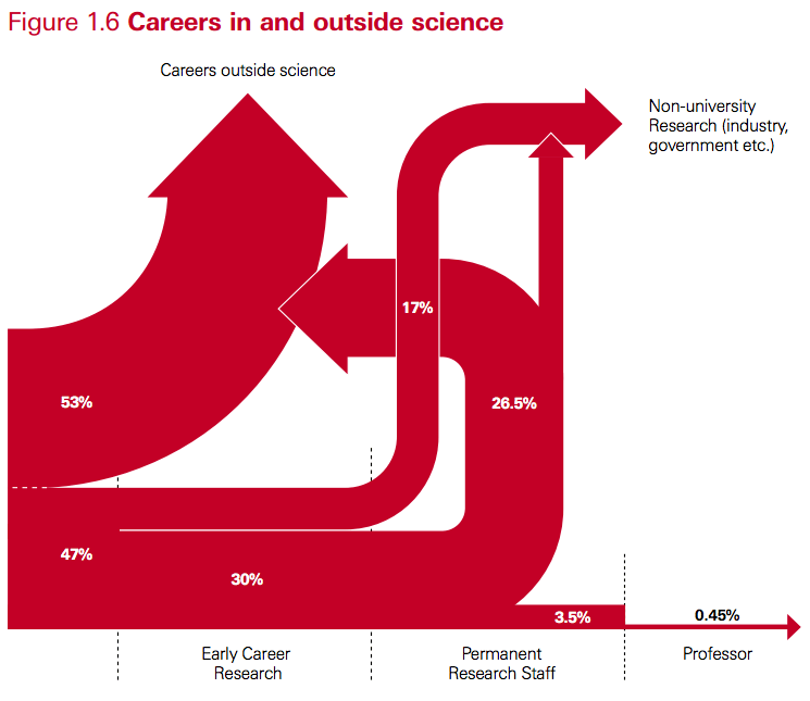
Yesterday, a friend posted this chart to Facebook, noting that the topic was “uk ph.d. graduate career paths” and that in their experience (as an academic in North America), the percentages looked pretty close. I share my friend’s concern about career options for PhDs, but looking at the diagram, the thing that stands out to me is how terrible it is — as a chart.

Screen shot 2013-11-10 at 11.57.09

Its source is a 2010 Royal Society policy report (PDF) entitled “The Scientific Century: securing our future prosperity”. In the original, Fig. 1.6 has a caption:

This diagram illustrates the transition points in typical academic scientific careers following a PhD and shows the flow of scientifically-trained people into other sectors. It is a simplified snapshot based on recent data from HEFCE[33], the Research Base Funders Forum[34] and from the Higher Education Statistics Agency’s (HESA) Annual Destinations of Leavers from Higher Education’ (DLHE) survey. It also draws on Vitae’s analysis of the DLHE survey[35]. It does not show career breaks or moves back into academic science from other sectors.

So what’s so bad about the chart? Some obvious issues:

  • It is unclear what goes in on the left and to a lesser degree what is covered by the end points. The report indicates in a footnote that the term “science” is used “as shorthand for disciplines in  the natural sciences, technology, engineering and mathematics,” but the three documents used for input categorise the fields in different ways, and there is no indication which fields exactly would have been selected.
  • Line thickness is not proportional to percentage weight. The 26.5% and 30% streams have the same thickness, and the 17% stream is much less  than half the thickness of either. The 3.5% stream is more than half the thickness of the 17% stream. 
  • Why does “Permanent Research Staff” not end in an arrow? And why does the arrow from “Permanent Research Staff” to “Careers Outside Science” bend backwards (to suggest it is a step back in one’s career, that is, an implicit value judgement?) and then not even merge with the output stream?
  • Does it really mean to suggest that no one goes from “Early Career Research” (that is, a post-doc) to “Career Outside Science” (or to industry research)? In my experience, watching post-docs, that is quite a common choice for post-docs precisely because non-academic jobs may be offering better pay and conditions, or because they don’t have a choice at that stage.

A graph like this is called a Sankey Diagram. They are very common to illustrate flows of energy, or of any quantity that is overall conserved (like here, the cohort of PhD. I wondered if I could make a better one (except for the flaws in content itself), even though I’ve never made one. I like to use R for data visualization tasks (or Python of course), so I quickly found out about a) Ramnath Vaidyanathan’s rather intriguing rCharts library, which provides interfaces from R to a variety of JavaScript plotting libraries and b) the implementation of the Sankey plugin for d3.js by someone called timelyportfolio. The integration is still a little rough for the newbie, but some crucial remarks at the end of  someone else’s tutorial got me started. (I’ve long been wanting to play with d3.js anyway, as it has impressive capabilities for geographic visualizations.)

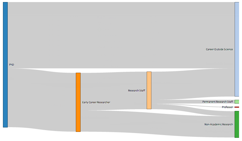
Here’s my version:

Screen shot 2013-11-10 at 11.56.56

Well, the fonts are too small. Click for full-sized image.

One advantage of plotting directly to HTML5/JavaScript is that sharing charts is extremely easy. As produced by d3.js, the chart isn’t too impressive, with several links overlapping. But as it is interactive, I manually cleaned it up and took the above screenshot.[1]

The cleaner chart illustrates most of the issues with the original one. Clearly it is unrealistic that any post-doc who later ends up in a career outside science or in non-academic research goes through another academic research staff position first. (And some go from post-doc directly to professor.) A bigger problem is the absence of differentiation by discipline. What does it mean that maybe 25% of STEM PhDs go through a period as temporary academic researchers before ending up outside science? I completely agree that this part of a researcher’s career is currently highly problematic in most Western countries (keywords: low compensation, high job insecurity, high expectations of personal investment in research), but there is a huge difference between a graduate from many engineering disciplines, where highly qualified people are finding highly satisfying “outside science” jobs, and fields where not staying in academia or public research after a PhD is the equivalent of a career change (think of astrophysics or pure mathematics). Also, the longer I think about it and look at some of the source documents (Vitae report, PDF) the more questions come up. Does Medicine count? Is teaching part of “career outside science”? What about higher education lectureships?

So in the end I remain with the feeling that no graph would have been more useful than this graph. The only thing it illustrates is confusion and uncertainty in the career paths, and as such, wouldn’t using a work of art to make the point have been more honest than what I can only call the illusion of science?

[1] For anyone interested, the code is here. It was also an opportunity to try out graphs in R.

Installing NCL on Ubuntu GNU/Linux 11.10

NCL stands for the NCAR Command Language, a free programming language that specializes in scientific data vizualisation. It is one of those rather idiosyncratic niche languages that few outside meteorology, climate science, oceanography or earth science have heard of but that can be a viable alternative to, say, Python with Nympy and Matplotlib, R, or for that matter the non-free but widespread Matlab.

It was during a pretty awesome NCL workshop that I started appreciating NCL more fully. Its main advantage, beyond the pretty powerful (and well documented) graphics capabilities, is that is provides a unified interface to some  unwieldy scientific and geospatial data formats. Coming from the world of commercial relational databases, it took me quite a while to understand how scientists think about data: a wide and deep topic for another post. For now, suffice it to say that scientific data often comes in large files that contain multiple series of data, plus metadata (data that describes either all or some of that data), and all need to be automatically processed. A typical task might be to read in such a file, retrieve several of the data series, select a sub-set of them (say, for some time span or some geographic area), calculate a new quantity, and plot the result on a map, with a proper map projection and latitude/longitudes. As I work daily with satellite data files (in formats that go by names such as HDF-EOS, NetCDF or HDF5), I appreciate a programming framework that swallows my downloaded GB and gives me this with a few lines of code and without costing an arm and a leg.

So for the scientist, trying out NCL might be a good idea, and on Mac OS X (10.6) this didn’t take more than a large binary download and a few clicks. Not so last weekend when I set up an Ubuntu system, unfortunately. So I apologize for this post becoming now very boring and describe how I got it to run and what decisions I made on the way.

0. The general approach

The following took place in a Virtualbox VM in order to create as reproducible a base as possible, that is a completely fresh install of Ubuntu 11.10 (Oneiric Ocelot) (the 32 bit desktop version).

What I’m describing is my third attempt, finally successful, at getting NCL up and running. Attempt 1 was to use the pre-compiled binaries, but the available 32-bit Debian Linux version just threw odd error messages that told me that at the very least some libraries and tools weren’t what it expected. This may have been fixable, but the task would have been frustrating and ultimately not very instructive.

Better to install from source, I thought, thinking I could use packages from the Ubuntu repositories for  most of the depenencies: libcairo, zlib or bison, or even widespread specialized stuff like GDAL (the Geopsatial Data Abstraction Layer software) are pretty standard, and the specialized file format libraries are available as well. However, this path also turned out to be fraught, mainly because the repository versions of the libraries related to these file types tended to not play nicely with each other, and also because the configuration file for the compilation of NCL itself expected certain libraires (hdf4, hdf5, netcdf, hdf-eos, hdf-eos5…) to be in certain locations relative to each other. I couldn’t get it right.

So at last here is what worked: Install only some of the dependencies, the unproblematic ones, from Ubuntu repositories, and install all of the finicky libraries and everything they  expect to be just-so through compilation from source. So here’s the recipe:

1. Install dependencies through the package manager

merian> sudo apt-get install build-essential gfortran csh ksh\
    flex bison openssl vim libcairo2-dev libjpeg62-dev libbz2-dev\
    libudunits2-dev libxaw7-dev libxt-dev libxft-dev libxpm-dev 
merian> sudo ln -s /usr/include/freetype2/freetype /usr/include/freetype

This takes care of: compilers, shells, tools; X11, graphics (including libpng and libjpeg), and some of the required compression libraries (bz2); and the Unidata Units package for unit transformations. It also corrects an odd discrepancy in where exactly the freetype library headers are expected by other source packages.

2. Download source code for the rest of the dependencies

There are a number of libraries NCL can optionally support or use. I decided not to install the whole kitchen sink, but to leave a few as an exercise to the reader, if needed: GRIB (a file format widely used for distributing meteorological data), Triangle (for triangular meshes used in climate modeling) and Vis5D+ (which I’ve never heard of). If you’re not interested in NASA satellite data, you can leave both of the HDF-EOS versions and HDF4 out as well. GDAL and PROJ4 are optional, too, but you really want nice mapping capabilities. This leaves the following tarballs.

3. Install dependencies from source

I’m following the NCAR instructions pretty closely and am installing in order: zlib first, then szip, libcurl and HDF5, which are needed by NetCDF. I was unable to persuade NetCDF to compile based on a mix of hand-compiled dependencies (in /usr/local/include) and Ubuntu header packets (in /usr/include), so all of the prerequisites had to be compiled, though some of their dependencies, in particular libjpeg and libpng, can be pre-installed. You may want to set the following environment variable, using setenv or export depending if you prefer a csh or bash type shell:

merian> export LD_LIBRARY_PATH=/usr/local/lib

Install zlib:

merian@ubuntu> ./configure --prefix=/usr/local
merian@ubuntu> make check; make install

Then, once zlib is installed, for example for libcurl, the configure command becomes:

merian@ubuntu> ./configure --prefix=/usr/local --with-zlib=/usr/local --with-pic

Pay attention to the libraries that you haven’t installed in /usr/local, and use –with-prefix=/usr in this case.

The biggest single task, and the only one where the NCAR/NCL site is incomplete, is putting NetCDF together. Very helpful are the installation instructions on the NetCDF site, both for the C libraries and the Fortran libraries. Do not worry about HDF4 support for NetCDF – we will give NCL HDF4 support through installing HDF4 directly.

Once you have NetCDF compiled and installed, the rest of the file formats come next: HDF4, HDF-EOS2 and HDF-EOS5. If you don’t need the last two, my suggestion is to simply not install support for them, but if you do follow the NCAR/NCL instructions to the letter. For HDF4, the most important point is not to forget –includedir=/usr/local/include/hdf as the software has its own version of the NetCDF header file (netcdf.h), which would overwrite the existing file. For HDF-EOS2, it is strongly advised not to use ./configure but to proceed as described and run bin/INSTALL-HDFEOS. The process involves manually editing makefiles and moving compiled libraries and header files to /usr/local/lib and /usr/local/include.

GDAL and PROJ4 are will typically be installed on any system that includes geospatial tools. The reason we install them from source is that GDAL comes with its own versions of HDF and other libraries, but needs to be linked against the same versions we built here. For the GDAL libraries, this configuration command worked well for me:

merian> ./configure --with-static-proj4=/usr/local --prefix=/usr/local \
    --without-pam --with-png=/usr --with-gif=internal \
    --with-libtiff=internal --with-geotiff=internal \
    --with-jpeg=/usr --with-libz=/usr/local \
    -with-sqlite3=no --with-expat=no --with-curl=no \
    --without-ld-shared --with-hdf4=no --with-hdf5=no\
    --with-pg=no --without-grib --with-freexl=no --with-geos=no

4. Install NCL

Downloading an NCL package requires a free registration at Earth System Grid/NCAR, which I’ve been told serves for NCAR to be able to count downloads and justify their funding. I do wonder if there isn’t a better way of achieving this.

Again, the instructions are nearly everywhere spot-on good. The process likes the environment variable NCARG to be set — I untar the source distribution, cd into the ncl_ncarg-[version] directory and run

merian> export NCARG=`pwd`

The SYSTEM_INCLUDE line returns “LINUX”, so that’s our makefile template. One change needs to be made in this file, regarding the Fortran compiler options:

#define FcOptions  -fPIC -fno-second-underscore -fno-range-check

Without the last option I got an arithmetic overflow error. It looked like it was only in a typecasting routine or other, but I guess I could have fixed that bug instead. In the configuration dialog, I used /usr/local/ncarg as the installation location, and I like then in the very end create symbolic links for the binary executables:

merian> ln -s /usr/local/ncarg/bin/* /usr/local/bin/

During the configuration dialogue, answer “yes” to all the optional dependencies you have compiled and “no” to those you don’t. And then compile. The make target “Everything” cleans out all previously compiled products, so takes longest if you have to fix a single error. “All” is faster, but what can happen is that the actual ncl executable may have got compiled but not moved to its final destination. So if your compilation output has no error but you can’t find the ncl executable, take a look in $NCARG/ni/src/ncl/. Otherwise it should be in /usr/local/ncarg/bin/ (or wherever your target location is.

Finally, test as described.

5. Final remarks

Frankly, I found this process painful. And I wonder why, much too often, we scientists put up with this — it’s not the first time that I’m seeing this. This is not a question of skills. I have the highest regard for the people at NCAR who maintain and develop NCL and provide free and high-quality support, thereby also spreading good coding practices and efficiency to newcomers. Maybe it’s the opposite: Because a typical computational scientists has the skills to deal with such an installation process, we don’t make the effort of fixing, say, the broken makefile of HDF-EOS2 once and for all, and don’t write install scripts that do away with the need to tell the software 592 times that we want it to be installed under /usr/local/ . Maybe there are license restrictions that would make it hard to repackage everything nicely, I don’t know. If so, we should make it clear that there’d be an advantage to getting rid of them.